
SUMIF is one of Google Sheets’ mathematical functions used to sum cells conditionally. The SUMIF function looks for a specified condition in a range of cells and then adds up the values that fit the provided condition.
For example, suppose you have a list of expenses in Google Sheets and want to total up only the charges that exceed a specified maximum number. Or you have a list of order items and their associated quantities, but you simply want to know the total order amount of a specific item. This is where the SUMIF function comes in.
The SUMIF function can sum items based on numeric conditions, text conditions, date conditions, wildcards, and empty and non-empty cells. SUMIF and SUMIFS are two Google Sheets functions for summarizing values depending on criteria. The SUMIF function adds numbers based on a single condition, but the SUMIFS function sums numbers based on many conditions.
This article will reveal to you how to utilize Google Sheets’ SUMIF and SUMIFS functions to total integers that match a specific condition (s).
The following are the guidelines for utilizing the SUMIFS function in Google Sheets:
• The SUMIFS function can handle a variety of circumstances. The SUMIF function, on the other hand, which we examined in our last post, only allows single conditions.
• Dates, messages, and numbers can all be used as criteria.
• The SUMIFS function accepts logical operators (>,>,=) as well as wildcards (*,?).
• An Equal number of rows and columns must appear in the additional ranges as in the sum range, but they do not have to be nearby. If you provide ranges that do not match, you will receive a #VALUE error.
• The SUMIF functions require a range and cannot be used with an array.
• Quotation marks should surround text strings in criteria, but cell references should not.
SUMIF in Google Sheets: 5 Easy Ways to Use It
SUMIF in Google Sheets can be used in five simple ways.
1. How to Use Google Sheets’ SUMIF Function with Numbers
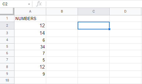
We will use the sample Google spreadsheet provided below to calculate the Google Sheets sum of values less than or equal 10. In cell C2, we shall compute the outcome.
Let’s look at how we may use the SUMIF function to calculate the sum.
Insert The Function Here
Enter the SUMIF function once you’ve selected the cell where you want to get the result.
The Google Sheets formula in our situation will be as follows.
=SUMIF(A2:A9,”<=10”)

In The Selected Cell, Enter The Formula
View the End Result
To show the total data in the spreadsheet, press the Enter key.

As you can see, the numbers that meet the stated requirement (6, 7, 5, and 9) are considered in the calculations.
2. Using the SUMIF Function with Text
Let’s look at how you can use the Google Sheets SUMIF function to compute the sum of text strings in sheets.
We shall take into account the sample sheet provided below.

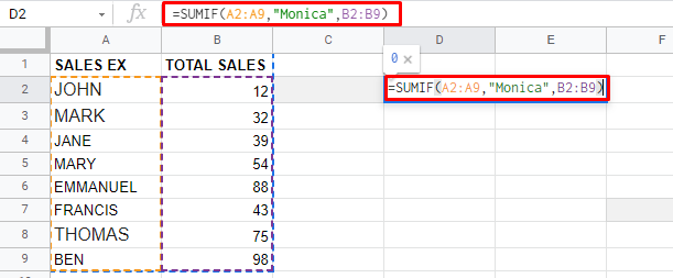
The goal is to compute Monica’s total sales and enter the result in cell D2.
Insert The Function Here
Create the function formula based on the supplied circumstance. The SUMIF formula in our situation will look like this.
=SUMIF(A2:A9,”Monica”,B2:B9)
View the End Result
To retrieve the result in the specified cell, press the Enter key.
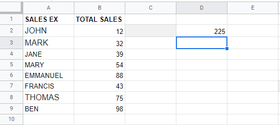
Take note of the distinction between the two cases. We didn’t need to specify the [sum range] section of the function in the first example, but we did in the second.
In this case, the SUMIF function first determined which cells in the first range matched the criteria and then chose the appropriate cell values from the second range’s cell reference, i.e., B2:B9.
It’s vital to notice that the [sum-range] portion is required when using the SUMIF function with certain text strings.
3. Using SUMIF With Dates
Let’s look at how we may use the SUMIF Google Sheets function in spreadsheets using dates.
Before we proceed with the procedure, we must first define the format for showing dates in Google Sheets, and you can do so by selecting Format from the menu bar.
Once you’ve settled on a date format, we’ll utilize the sample sheet provided below to help you understand the concept.
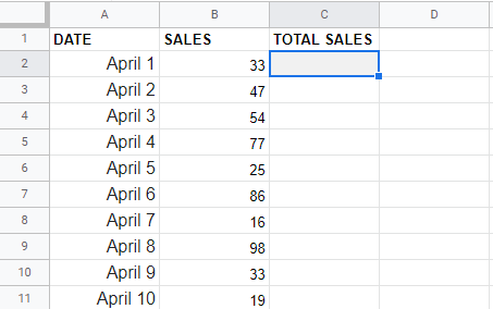
The main goal is to compute the total sales in column B from March 1 to April 5 in cell C2.
Input The Formula
To begin, create the function and enter it into the appropriate cell. In the example, the formula is as follows.
=SUMIF(A2:A11,”<“&DATE(2021,4,5),B2:B11)
Take note of the DATE function’s default syntax here: (year, month, day). You must enter the date using the DATE function syntax.
It would be best to use the ampersand(&) symbol to connect the” “operator to the DATE function.

View the End Result
When you press the Return key, the answer will appear in the selected cell.

The SUMIF function returned the sum of all sales made before April 5 based on the specified formula; the values for April 5 were not considered in the function. If you want the SUMIF function to take it into account, modify the operator in the equation from “<” to “=<“.
4. Using SUMIF With Wildcards
Although it is not needed, you can utilize Wildcards with the SUMIF function.
We’ll utilize the sample sheet provided below for this example.

The fundamental goal is to compute the total quantity of all TV-related products. Let’s look at an example to see how we can do that.
Input The Formula
To begin, select the cell, in this case, C2, and enter the SUMIF function as shown below.
=SUMIF(A2:A7,”TV*”,B2:B7)
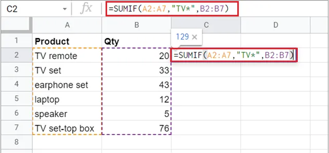
Look at the outcome
Now, press the Return key to see the results in the cell you’ve chosen. In this example, the algorithm considers values from SUMIF cells B2, B3, and B7 because their corresponding cells in column A contain the phrase ‘TV.’

The asterisk symbol ‘*’ represents a WildCard character. This single character instructs Google Sheets to search for all cell values in a specified data range containing a specific word. WildCards do not require an exact match, only the existence of the provided phrase.
5. Using the SUMIF Function on Blank and Non-Blank Cells
SUMIF Google Sheets can be used with both blank and non-blank cells. Let’s look at this with the help of the sample Google sheet provided below.

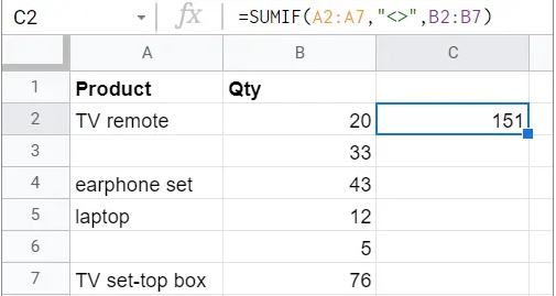
You must now calculate the sum of just non-blank cells in cell C2.
The SUMIF formula comes into play.
In the selected cell, enter the Google Sheets SUMIF formula. It will be as follows.
=SUMIF(A2:A7,”<>”,B2:B7)
The non-blank cells are denoted by the logical operator “<>”.

View the End Result
To view the sum value in the selected cell, press the Enter key.
If you want to check the total for the corresponding cell values of a blank cell, you can use the “logical operator instead of the “<>” logical operator.

Because the matching cells in column A are blank, the SUMIF function considered cell values from B3 and B6 in this example. You can use conditional formatting to highlight the cell range that SUMIF has considered in its calculations for even more detailed visualization.
Users must also be aware that the SUMIF formula cannot be utilized within an array formula. The SUMIF formula is most commonly used in a Google Sheets budget spreadsheet to calculate values according to a given text string.
Conclusion
SUMIF in Google Sheets lets users compute the sum of values in cells that meet a single, specific, or numerous conditions. It can be used with data that includes text strings and numbers and numbers, and it also happens to be one of the essential data analysis functions in Google Sheets.
If you wish to avoid problems when using the SUMIF function in Google Sheets, you should keep a few things in mind. If you wish to sum values that fulfill numerous conditions rather than just one, use the SUMIF formula.